Deciphering cell-cell communication in single-cell transcriptomics data

Cell-cell communication plays a crucial role in coordinating cellular activities and maintaining the overall functionality of multicellular organisms. It allows cells to transmit signals, exchange information, and coordinate their behaviors, ultimately contributing to essential biological processes such as development, immune response, and tissue homeostasis. In this context, inferring cell-cell interactions from gene expression data becomes valuable for unraveling the multiple roles and coordination processes that cells perform within multicellular systems. In this notebook, main concepts and a general computational workflow will be covered, then hands-on activities will be performed using LIANA, a flexible tool implementing multiple state-of-the-art methods to study cell-cell interactions.

Install the required libraries


# Download a shell script to add CRAN repositories to Ubuntu Jammy
download.file("https://github.com/eddelbuettel/r2u/raw/master/inst/scripts/add_cranapt_jammy.sh",
              "add_cranapt_jammy.sh")
# Change the file permission to make it executable
Sys.chmod("add_cranapt_jammy.sh", "0755")
# Execute the shell script
system("./add_cranapt_jammy.sh")

# Enable Binary Package Manager (bspm) to manage system and CRAN packages
bspm::enable()
options(bspm.version.check=FALSE)

We will create an R function to performs system calls


# Define a function to execute shell commands and print the output
shell_call <- function(command, ...) {
  result <- system(command, intern = TRUE, ...)
  cat(paste0(result, collapse = "\n"))
}

Install required libraries


# Install required R packages
install.packages("R.utils")
# Install Seurat Wrappers from GitHub (commented out)
# remotes::install_github('satijalab/seurat-wrappers@d28512f804d5fe05e6d68900ca9221020d52cf1d', upgrade=F)

# Install BiocManager if not already installed
if (!require("BiocManager", quietly = TRUE))
    install.packages("BiocManager", quiet = T)

# Install Harmony and LIANA from GitHub
install.packages("harmony")
remotes::install_github('saezlab/liana', upgrade=F)

Introduction

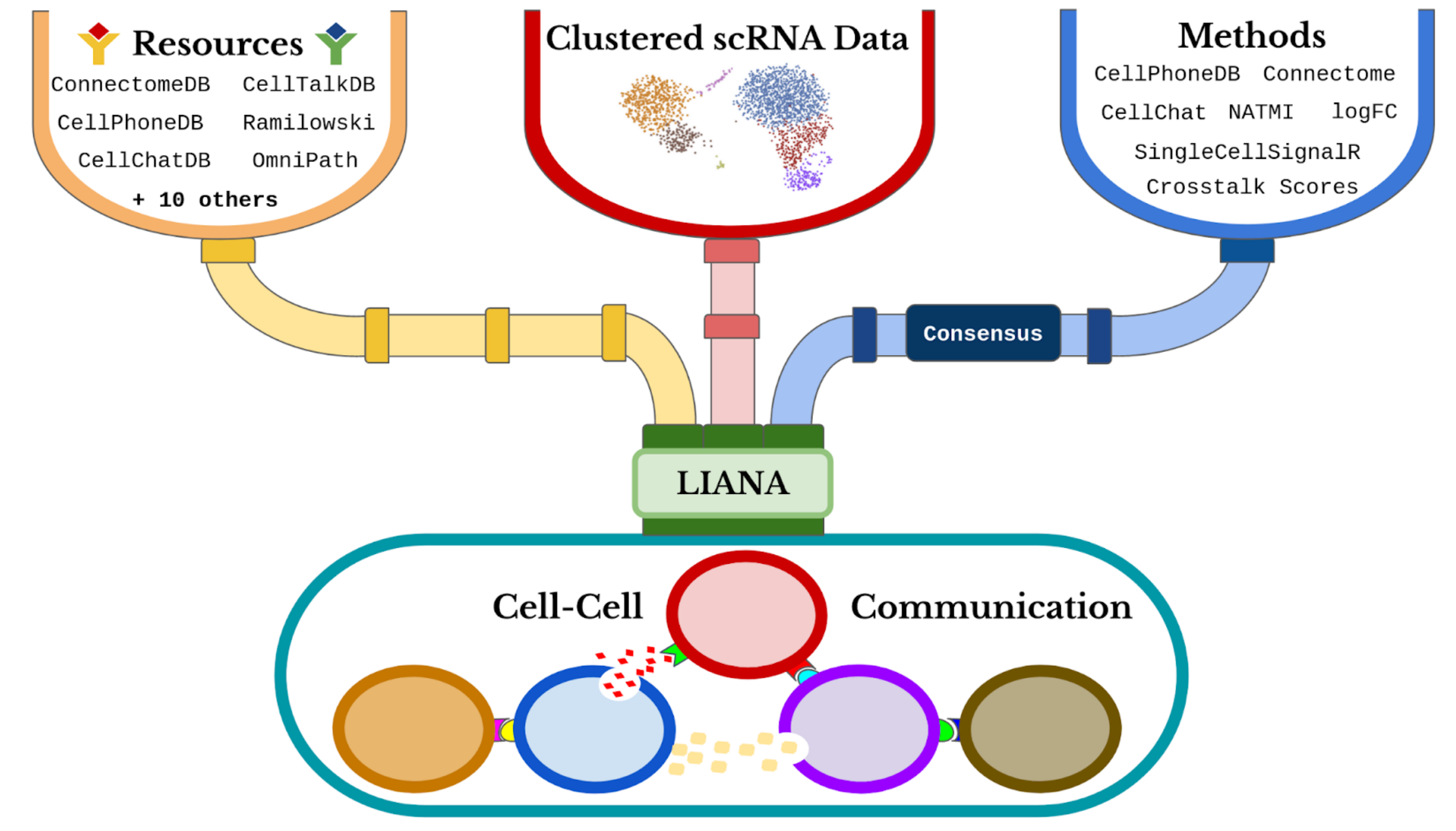
LIANA (Ligand-Receptor Inference Analysis) offers a variety of statistical methods to infer ligand-receptor interactions from single-cell transcriptomic data, using prior knowledge. This notebook aims to demonstrate how to use LIANA in a basic way with our data of interest.

Steps for Using LIANA:

1. Data Preparation:

Upload your single-cell transcriptomic data in the appropriate format.

Make sure the data is normalized and annotated correctly.

2. LIANA Installation and Import:

Install the LIANA package, if it is not already installed, using the command pip install liana.

Import the package into your notebook with import liana.

3. LIANA Configuration:

Set the parameters required for the analysis, such as the cell type and signaling pathways of interest.

Use LIANA-specific functions to define the ligand-receptor interactions you want to investigate.

4. Analysis Execution:

Perform the analysis using the statistical methods available in LIANA.

Analyze results to identify significant interactions between ligands and receptors in your samples.

5. Result Interpretation:

Visualize results using built-in visualization tools or export data for further analysis.

Interpret identified interactions in the biological context of your study.


# Install the Seurat package for single-cell analysis
install.packages("Seurat")


# Load necessary libraries for data manipulation and analysis
library(tidyverse)  # Collection of packages for data science
library(magrittr)   # Pipe operator
library(liana)      # Cell-cell communication analysis
library(Seurat)     # Single-cell RNA-seq analysis

In this section, we will showcase all the methods implemented by LIANA from various tools. Each method infers relevant ligand-receptor interactions based on different assumptions. Typically, each method returns two scores for each ligand-receptor pair:

1.Magnitude (Strength) Score: This score indicates the strength of the interaction.

2.Specificity Score: This score reflects how specific the interaction is to a given pair of cell identities.


# Show available methods in the current R session
show_methods()

The different resources of ligand-receptor interactions can be found here. The consensus integrates all the other resources.


# Show available resources in the current R session
show_resources()

Loading data

Here we load our data of interest to study cell-cell communicaton.


# Download the COVID-19 dataset (RDS file) from Dropbox
download.file("https://www.dropbox.com/scl/fi/1ysew52kr8o2riahzubcw/BALF-COVID19-Liao_et_al-NatMed-2020.rds?rlkey=tg3tpn8la6oth25wvx3a22qt9&dl=1", "COVID.rds")


# Read the RDS file into a variable called 'testdata'
testdata <- readRDS('COVID.rds')


# Display an overview of the 'testdata' structure
testdata %>% dplyr::glimpse()


# This specific condition 'group == "S" ' is being used to filter the rows. Only those rows where the group column value is equal to "S" will be included in the subset.
testdata <- subset(x = testdata, subset = group == "S")


# This function is used to get or set the identifiers of an object. The new columm is named "celltype"
Idents(testdata) <- "celltype"


# Normalize the single-cell RNA-seq data using Seurat
testdata <- Seurat::NormalizeData(testdata, verbose = FALSE)


    # Display the structure of the processed dataset
testdata %>% dplyr::glimpse()

Running LIANA

To run LIANA, you can choose from any of the methods it supports. In this example, we will use the CellPhoneDB implementation.

The liana_wrap function invokes multiple methods, each operating with the provided resource(s). If no specific method is specified, liana_wrap will execute all methods implemented in LIANA. Additionally, the consensus resource is used by default.


cpdb_result <- liana_wrap(testdata, # This function of the LIANA package is used to perform cell-cell interaction analyses using different methods
                          method = 'cellphonedb',
                          resource = c('CellPhoneDB'), # Specifies that the CellPhoneDB method will be used
                          permutation.params = list(nperms=100, # Defines the permutation parameters. nperms=100: Number of permutations
                                                    parallelize=FALSE, # Indicates whether execution should be parallelized
                                                    workers=4), # Number of workers to use if execution were parallelized
                          expr_prop=0.05) # Minimum proportion of expression to consider an interaction as valid


# Display the structure of the CellPhoneDB interaction results
dplyr::glimpse(cpdb_result)

To run LIANA using multiple methods simultaneously, you can specify the desired methods in the method parameter. In this example, we will use CellPhoneDB, NATMI, SingleCellSignalR (sca), and the logFC approach.


# Run a more complex interaction analysis using multiple methods
complex_test <- liana_wrap(testdata,
                           method = c('cellphonedb', 'natmi', 'sca', 'logfc'),
                           resource = c('CellPhoneDB'))  # Use CellPhoneDB resource


# Display the structure of the complex interaction results
dplyr::glimpse(complex_test)

One of the key features of LIANA is that it can compute a consensus ranking of the prediction of all methods employed to analyze cell-cell communication. By using the function liana_aggregate() we can use all the results from every method used in the previous step.


# Aggregate interaction results across multiple methods
liana_consensus <- complex_test %>% liana_aggregate()


# Display the structure of the aggregated interaction results
dplyr::glimpse(liana_consensus)

Visualization and interpretation

Dotplots can be generated to easily interpret important ligand-receptor pairs used by sender-receiver cell pairs.

Here, we preprocess the results of CellPhoneDB, then plot them. A filter to use only significant cases is applied (P-value < 0.05).


cpdb_int <- cpdb_result %>%
  # Only keep interactions with p-val <= 0.05
  filter(pvalue <= 0.05) %>% # This reflects interactions `specificity`
  rank_method(method_name = "cellphonedb", mode = "magnitude") %>% # Then rank according to `magnitude` (lr_mean in this case)
  distinct_at(c("ligand.complex", "receptor.complex")) %>% # Keep top 20 interactions (regardless of cell type)
  head(20)


# Options(repr.plot.height = 12, repr.plot.width = 9)
# Plot cell-cell interactions using LIANA's dotplot function
scPlot <- cpdb_result %>%  
          inner_join(cpdb_int, # Keep only the interactions of interest
                    by = c("ligand.complex", "receptor.complex")) %>%  # Invert size (low p-value/high specificity = larger dot size), add a small value to avoid Infinity for 0s
          mutate(pvalue = -log10(pvalue + 1e-10)) %>% # Transforms the p-value by taking the negative log10
          liana_dotplot(source_groups = c("Epithelial"), # Creates a dot plot for the specified source and target groups, and specifies the source group
                        target_groups = c("Macrophages", "NK", "B", "T", "Neutrophil"), # Specifies the target groups.
                        specificity = "pvalue", # Uses the p-value for dot size specification.
                        magnitude = "lr.mean", # Uses the mean log ratio for the dot color
                        show_complex = TRUE,
                        size.label = "-log10(p-value)") + theme(axis.text.x = element_text(angle = 90))
scPlot
# Save the plot as an image file
ggsave("01-liana_dotplot.png", plot = scPlot, bg = "white", dpi = 600, width = 16, height = 9)

Similarly, we can explore the consensus results.


# Options(repr.plot.height = 12, repr.plot.width = 9)
# Plot top 20 interactions from aggregated LIANA results
scPlot <- liana_consensus %>%
          liana_dotplot(source_groups = c("Macrophages"),
                        target_groups = c("Macrophages", "NK", "B", "T", "Neutrophil"),
                        ntop = 20) + theme(axis.text.x = element_text(angle = 90))
scPlot
# Save the plot
ggsave("02-liana_dotplot.png", plot = scPlot, bg = "white", dpi = 600, width = 16, height = 9)

Overall potential of cells to communicate can be computed. Here, we can count the number of significant/important interactions. Then, they can be visualized through a heatmap.

Similarly, we can compare the CellPhoneDB vs consensus results.


# Filter interactions with p-value ≤ 0.05 and plot frequency heatmap
liana_trunc <- cpdb_result %>% filter(pvalue <= 0.05)

# Generate and save heatmap
# png("03-heat_freq.png", bg = "white")
heat_freq(liana_trunc)
# dev.off()


# Filter consensus interactions with aggregate rank ≤ 0.01 and plot heatmap
liana_trunc <- liana_consensus %>% filter(aggregate_rank <= 0.01)

# Generate and save heatmap
# png("04-heat_freq.png", bg = "white")
heat_freq(liana_trunc)
# dev.off()

Extra questions:

How different are the results between two methods of your choice?

Why can this happen?